Statistics

Introduction

This is majorl ## Standard Definitions

Expected Value $\mathbb{E}[X]$ is given by

$$\mathbb{E}[X]={\int }_{-\mathrm{\infty }}^{\mathrm{\infty }}xf(x)dx$$ Variance$Var(X)$ is given by

$$Var(X)=\mathbb{E}(X^2)-\mathbb{E}{(X)}^2$$ $$Var(X)={\int }_{-\mathrm{\infty }}^{\mathrm{\infty }}(x-\mathbb{E}[X]{)}^2{f}_X(x)dx$$ Higher Moments $\mathbb{E}(X^n)$ is given by

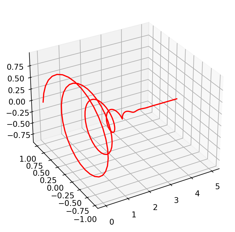
$$\mathbb{E}(X^n)={\int }_{-\mathrm{\infty }}^{\mathrm{\infty }}{x}^n{f}_X(x)dx$$ Characteristic function(CHF) ${\varphi }_X(u)$ for $u\in \mathbb{R}$ is given by

$${\varphi }_X(u)=\mathbb{E}[e^{iuX}]={\int }_{-\mathrm{\infty }}^{\mathrm{\infty }}{e}^{iuX}f(x)dx$$

Moment generating function${\mathcal{M}}_X(u)$ is given by $${\mathcal{M}}_X(u)={\varphi }_X(-iu)=\mathbb{E}[e^{uX}]={\int }_{-\mathrm{\infty }}^{\mathrm{\infty }}{e}^{ux}f(x)dx$$ Cumulant characteristic function ${\zeta }_X(u)$ is given by $${\zeta }_X(u)=log\mathbb{E}[e^{iux}]=log{\varphi }_X(u)$$

Central moments$ _l$ is given by $\mathbb{E}[(X-\mu {)}^l]$

Skewness $S(x)$ and Kurtosis $K(x)$ are the normalised $3^{rd}$ and $4^{th}$ central moments of a distribution respectively. The normalization factors are ${\sigma }^3$ and ${\sigma }^4$ respectively where $\sigma$ is the standard deviation of X.

The quantity $K(x)-3$ is called the excess kurtosis since $K(x)=3$ is the kurtosis for a normal distribution.

Let $\{x_1,x_2,x_3....x_T\}$ be a random sample of X with T observations

Sample Mean${\hat{\mu }}_x$ is given by $$\frac{\sum _{t=1}^T{x}_t}{T}$$ Sample Variance${\hat{\sigma }}_x$ is given by $$\frac{\sum _{t=1}^T(x_t-{\hat{\mu }}_x{)}^2}{T-1}$$ Sample Skewness${\hat{S}}_x$ is given by $$\frac{\sum _{t=1}^T(x_t-{\hat{\mu }}_x{)}^3}{(T-1){\hat{\sigma }}_x^3}$$ Sample Kurtosis${\hat{K}}_x$ is given by $$\frac{\sum _{t=1}^T(x_t-{\hat{\mu }}_x{)}^4}{(T-1){\hat{\sigma }}_x^4}$$

Univaiate Distributions

Normal Distribution

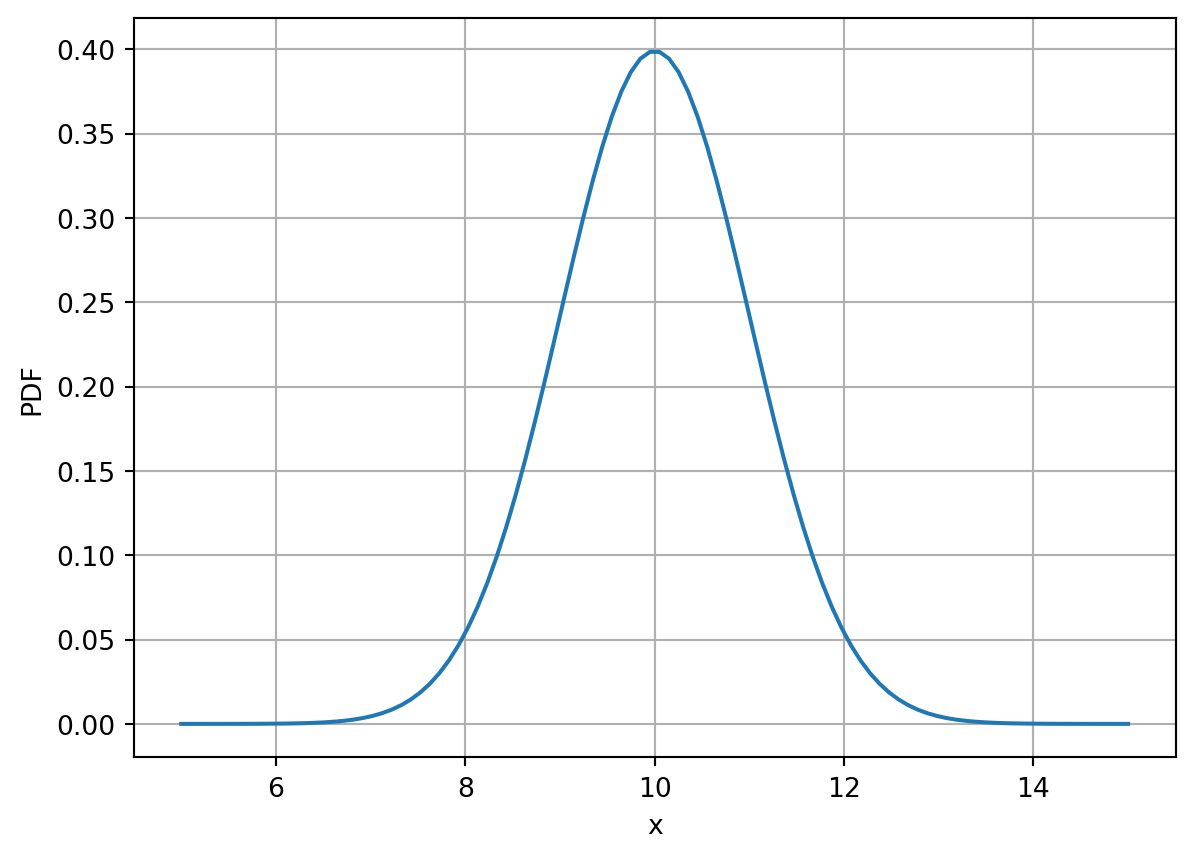
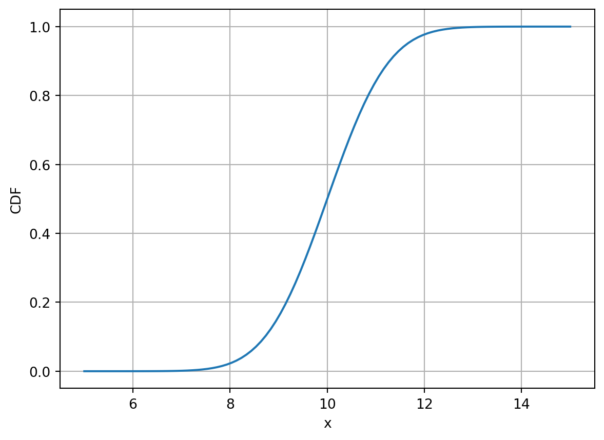
A random variable $X$ is said to be normally distrbuted if it has a probability density function as follows

$$f_X(x)=\frac{1}{\sigma \sqrt{2\pi }}{e}^{-\frac{1}{2}(\frac{x-\mu }{\sigma }{)}^2}$$

It is a continous probability distribution

$\mu$ and $\sigma$ are the mean and variance of the distribution respectively

The case where $\mu =0$ and $\sigma =1$ is called standard normal distribution and its PDF is given by $$f_X(x)=\frac{1}{\sqrt{2\pi }}{e}^{\frac{-x^2}{2}}$$

import numpy as np
import math 
import matplotlib.pyplot as plt
import scipy.stats as st
from mpl_toolkits import mplot3d


def plotNormalPDF_CDF_CHF(mu ,sigma):
    i = complex(0,1)
    chf = lambda u : np.exp(i*mu*u -(sigma**2)*u*u/2)
    pdf = lambda x : st.norm.pdf(x,mu,sigma)
    cdf = lambda x : st.norm.cdf(x,mu,sigma)
    
    x = np.linspace(5,15,100)
    u = np.linspace(0,5,250)
    print(type(pdf))
    # figure 1 ,PDF
    plt.figure(1)
    plt.plot(x,pdf(x))
    plt.grid()
    plt.xlabel('x')
    plt.ylabel('PDF')
  
    # figure 2 ,CDF
    plt.figure(2)
    plt.plot(x,cdf(x))
    plt.grid()
    plt.xlabel('x')
    plt.ylabel('CDF')
  
    #  figure 3 ,CHF
  
    plt.figure(3)
    ax = plt.axes(projection = '3d')
    chfV = chf(u)
  
    x = np.real(chfV)
    y = np.imag(chfV)
    ax.plot3D(u,x,y,'red')
    ax.view_init(30 ,-120)
    
plotNormalPDF_CDF_CHF(10,1)

<class 'function'>

Log Normal Distibution

A random Variable $X$ is said to have log normal distibution if $Y=\ln X$ and $Y$ is normally distributed.

The PDF of log normal distribution is given by

$$f_X(x)=\frac{1}{x\sigma \sqrt{2\pi }}{e}^{(-\frac{(\ln x-\mu {)}^2}{2{\sigma }^2})}$$ where $\mu$ and $\sigma$ are the mean and variance of $Y(\ln X)$ respectively.

Hence the mean ${\mu }^{\ast }$ and variance ${\sigma }^{\ast }$ of X are as follows

$${\mu }^{\ast }=e^{\mu +\frac{1}{2}{\sigma }^2}$$ $${\sigma }^{\ast }=e^{2\mu +2{\sigma }^2}-e^{2\mu +{\sigma }^2}$$ Important thing to note here is that $x$ can take values in $(0,\mathrm{\infty })$ only.

Multivariate Distributions

Correlation

The correlation coefficient between two random variables $X$ and $Y$ is defined as $${\rho }_{x,y}=\frac{Cov(X,Y)}{\sqrt{Var(X)Var(Y)}}=\frac{E[(X-{\mu }_x)(Y-{\mu }_y)]}{\sqrt{E(X-{\mu }_x{)}^{2}E(Y-{\mu }_y{)}^2}}$$

The sample correlation is given by $${\hat{\rho }}_{x,y}=\frac{\sum _{t=1}^T(x_t-\overline{x})(y_t-\overline{y})}{\sqrt{\sum _{t=1}^T(x_t-\overline{x})\sum _{t=1}^T(y_t-\overline{y})}}$$

Two-dimensional densities.

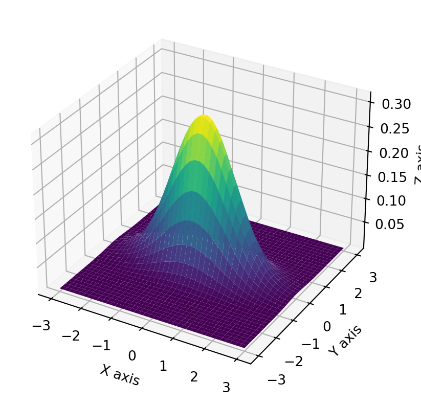
The joint CDF of two random variables ,$X$ and $Y$ ,is the function $F_{X,Y}(.,.):{\mathbb{R}}^2\to [0,1]$,which is defined by:

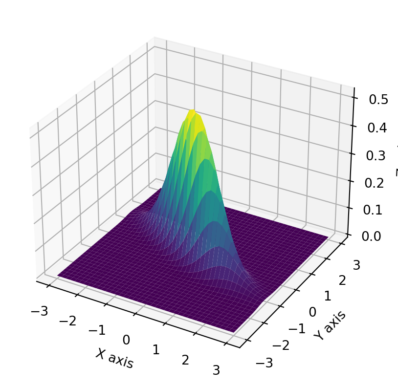
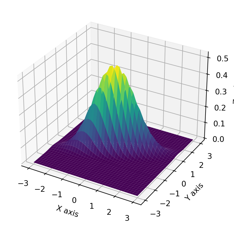
$$F_{X,Y}(x,y)=\mathbb{P}[X\le x,Y\le y]$$ If $X$ and $Y$ are continous variables, then the joint PDF of X and Y is a function of $$f_{X,Y}(x,y)=\frac{{\partial }^2{F}_{X,Y}(x,y)}{\partial x\partial y}$$ Bivariate Normal density functions

$X=[X,Y{]}^T$ and $$X\sim \mathcal{N}(\left[\begin{array}{c}0\\ 0\end{array}\right],\left[\begin{array}{c}1,\rho \\ \rho ,1\end{array}\right])$$

import numpy as np
import matplotlib.pyplot as plt
#from matplotlib.mlab import bivariate_normal bivariate_normal seems to be deprecated

def bivariate_normal(X, Y, sigmax=1.0, sigmay=1.0,
                     mux=0.0, muy=0.0, sigmaxy=0.0):
    """
    Bivariate Gaussian distribution for equal shape *X*, *Y*.
    See `bivariate normal
    <http://mathworld.wolfram.com/BivariateNormalDistribution.html>`_
    at mathworld.
    """
    Xmu = X-mux
    Ymu = Y-muy

    rho = sigmaxy/(sigmax*sigmay)
    z = Xmu**2/sigmax**2 + Ymu**2/sigmay**2 - 2*rho*Xmu*Ymu/(sigmax*sigmay)
    denom = 2*np.pi*sigmax*sigmay*np.sqrt(1-rho**2)
    return np.exp(-z/(2*(1-rho**2))) / denom

def BivariateNormalPDFPlot():
  # Number of points in each direction
      n = 40;
      
      # parameters
      mu_1 = 0;
      mu_2 = 0;
      sigma_1=1;
      sigma_2=0.5;
      rho1=0.0
      rho2=-0.8
      rho3=0.8
      
      x = np.linspace(-3.0,3.0,n)
      y = np.linspace(-3.0,3.0,n)
      X,Y =np.meshgrid(x,y)
      Z = lambda rho:bivariate_normal(X,Y,sigma_1,sigma_2,mu_1,mu_2,rho*sigma_1*sigma_2)
      
      fig =plt.figure(1)
      ax = fig.add_subplot(projection= '3d')
      ax.plot_surface(X, Y, Z(rho1),cmap='viridis',linewidth=0)
      ax.set_xlabel('X axis')
      ax.set_ylabel('Y axis')
      ax.set_zlabel('Z axis')
      plt.show()
      
      fig =plt.figure(2)
      ax = fig.add_subplot(projection= '3d')
      ax.plot_surface(X, Y, Z(rho2),cmap='viridis',linewidth=0)
      ax.set_xlabel('X axis')
      ax.set_ylabel('Y axis')
      ax.set_zlabel('Z axis')
      plt.show()
      
      fig =plt.figure(3)
      ax = fig.add_subplot(projection= '3d')
      ax.plot_surface(X, Y, Z(rho3),cmap='viridis',linewidth=0)
      ax.set_xlabel('X axis')
      ax.set_ylabel('Y axis')
      ax.set_zlabel('Z axis')
      plt.show()
  
BivariateNormalPDFPlot()

Hypothesis Testing

t-statistic is the ratio of departure of the estimated value of a paramater from its hypothesized value to it’s standard error.

It is used when the sample size is small or the population standard deviation is unknown.

Let $\hat{\beta }$ be an estimator of parameter $\beta$ in some statistical model. Then the t-statistic is given by $$t_{\hat{\beta }}=\frac{\hat{\beta }-{\beta }_0}{s.e(\hat{\beta })}$$ where $s.e(\hat{\beta })$ is the standard error of the estimator $\hat{\beta }$ for $\beta$ and ${\beta }_0$ is a non-random , know constant , which may or maynot match actual unknow parameter value $\beta$