Hands-On Machine Learning with Scikit-Learn ,Keras and Tensorflow

Introduction

A pure code based implementation with necessary mathematical formulations included.

End to End machine Learning

Performance Measure

Root Mean Square Error RMSE(\textbf{X},h)= \sqrt{\frac{\sum_{i = 1}^{m}{(h{(x^{(i)})- y ^{(i)}}})^2}{m}} m- is the number of instances in the datasets you are measuring the RMSE on
x^{(i)}- is the vector of all teh feature values of the i^{th} instance in the dataset
y^{(i)}- is its label
\textbf{X}- is the matrix containing all the feature value of all the instances in the dataset. x^{(i)} transpose is the i^{th}-row in \textbf{X}
h - is the system’s prediction function also called as hypothesis. It is also represented by \hat{y} where \hat{y}^{(i)} = h(x^{(i)})
RMSE(\textbf{X},h)- is the cost function measured on the set of examples using the hypothesis h

Mean absolute Error MAE(\textbf{X},h)= \frac{\sum_{i = 1}^{m}{|h{(x^{(i)})- y ^{(i)}}}|}{m}

The difference between these two performance measure is how the norm is caculated. RSME makes use of \mathcal{l}_2 norm while MAE makes use of \mathcal{l}_1 norm.

Download the DATA

import os 
import tarfile
import urllib

Download_Root = "https://raw.githubusercontent.com/ageron/handson-ml2/master/"
Housing_Path = os.path.join("Data","housing") # for creating your local directory with DATA as main directory and housign as sub directory
Housing_URL = Download_Root + "datasets/housing/housing.tgz"

def fetch_housing_data(housing_url = Housing_URL,housing_path = Housing_Path):
    os.makedirs(housing_path,exist_ok = True)# Will create a directory with name at housing path , exist_ok will check if it already exist , if yes leaving it unaltered
    tgz_path = os.path.join(housing_path,"housing.tgz")
    urllib.request.urlretrieve(housing_url,tgz_path)
    housing_tgz = tarfile.open(tgz_path)
    housing_tgz.extractall(path=housing_path)
    housing_tgz.close()
    
fetch_housing_data() # call the function

import pandas as pd

def load_housing_data(housing_path = Housing_Path):
    csv_path = os.path.join(housing_path,"housing.csv")
    return pd.read_csv(csv_path)

housing = load_housing_data()
housing.head()

	longitude	latitude	housing_median_age	total_rooms	total_bedrooms	population	households	median_income	median_house_value	ocean_proximity
0	-122.23	37.88	41.0	880.0	129.0	322.0	126.0	8.3252	452600.0	NEAR BAY
1	-122.22	37.86	21.0	7099.0	1106.0	2401.0	1138.0	8.3014	358500.0	NEAR BAY
2	-122.24	37.85	52.0	1467.0	190.0	496.0	177.0	7.2574	352100.0	NEAR BAY
3	-122.25	37.85	52.0	1274.0	235.0	558.0	219.0	5.6431	341300.0	NEAR BAY
4	-122.25	37.85	52.0	1627.0	280.0	565.0	259.0	3.8462	342200.0	NEAR BAY

housing.info()

<class 'pandas.core.frame.DataFrame'>
RangeIndex: 20640 entries, 0 to 20639
Data columns (total 10 columns):
 #   Column              Non-Null Count  Dtype  
---  ------              --------------  -----  
 0   longitude           20640 non-null  float64
 1   latitude            20640 non-null  float64
 2   housing_median_age  20640 non-null  float64
 3   total_rooms         20640 non-null  float64
 4   total_bedrooms      20433 non-null  float64
 5   population          20640 non-null  float64
 6   households          20640 non-null  float64
 7   median_income       20640 non-null  float64
 8   median_house_value  20640 non-null  float64
 9   ocean_proximity     20640 non-null  object 
dtypes: float64(9), object(1)
memory usage: 1.6+ MB

housing["ocean_proximity"].value_counts()

<1H OCEAN     9136
INLAND        6551
NEAR OCEAN    2658
NEAR BAY      2290
ISLAND           5
Name: ocean_proximity, dtype: int64

housing.describe()

	longitude	latitude	housing_median_age	total_rooms	total_bedrooms	population	households	median_income	median_house_value
count	20640.000000	20640.000000	20640.000000	20640.000000	20433.000000	20640.000000	20640.000000	20640.000000	20640.000000
mean	-119.569704	35.631861	28.639486	2635.763081	537.870553	1425.476744	499.539680	3.870671	206855.816909
std	2.003532	2.135952	12.585558	2181.615252	421.385070	1132.462122	382.329753	1.899822	115395.615874
min	-124.350000	32.540000	1.000000	2.000000	1.000000	3.000000	1.000000	0.499900	14999.000000
25%	-121.800000	33.930000	18.000000	1447.750000	296.000000	787.000000	280.000000	2.563400	119600.000000
50%	-118.490000	34.260000	29.000000	2127.000000	435.000000	1166.000000	409.000000	3.534800	179700.000000
75%	-118.010000	37.710000	37.000000	3148.000000	647.000000	1725.000000	605.000000	4.743250	264725.000000
max	-114.310000	41.950000	52.000000	39320.000000	6445.000000	35682.000000	6082.000000	15.000100	500001.000000

%matplotlib inline 
import matplotlib.pyplot as plt
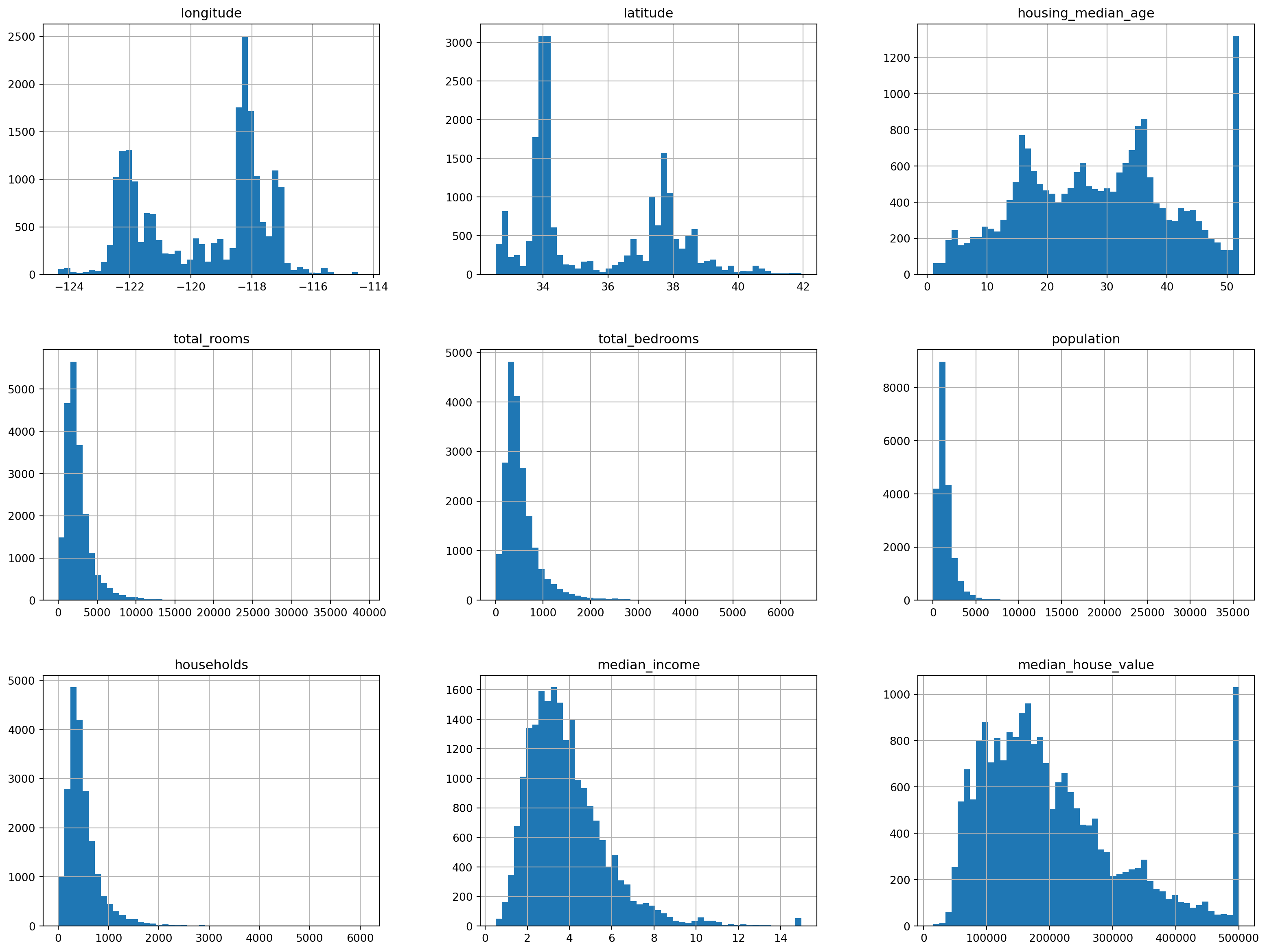
housing.hist(bins = 50 ,figsize = (20,15))

array([[<AxesSubplot: title={'center': 'longitude'}>,
        <AxesSubplot: title={'center': 'latitude'}>,
        <AxesSubplot: title={'center': 'housing_median_age'}>],
       [<AxesSubplot: title={'center': 'total_rooms'}>,
        <AxesSubplot: title={'center': 'total_bedrooms'}>,
        <AxesSubplot: title={'center': 'population'}>],
       [<AxesSubplot: title={'center': 'households'}>,
        <AxesSubplot: title={'center': 'median_income'}>,
        <AxesSubplot: title={'center': 'median_house_value'}>]],
      dtype=object)

Few point about the data

The median income is capped at 15 for higher median incomes and at 0.5 for lower median incomes. The numbers are denominated in $10000 i.e 3 in the chart represents 30,000 USD
The housing median age and median house value were also capped. Since median house value is our target variable this is a source of a problem.The prediction might never go beyond the capped limit.
The attributes have different scales
Many of the histograms are tail-heavy. Important to normalize the data as some machine learning algorithims might fail to detect patterns effectively

Creating a test set and train set

import numpy as np
np.random.seed(50)# will always give the same test set and train set 
def split_train_test(data,test_ratio):
    shuffled_indices = np.random.permutation(len(data))
    test_set_size = int(len(data)*test_ratio)
    test_indices = shuffled_indices[:test_set_size]
    train_indices = shuffled_indices[test_set_size:]
    return data.loc[train_indices] ,data.loc[test_indices]

train_set , test_set = split_train_test(housing,0.2)
print(len(train_set))
print(len(test_set))

16512
4128